
In the post on breaking ciphers, I asserted that the bag of letters model (a.k.a. the "random monkey typing" model) was the best one for checking if a piece of text is close to English. Is that true?
But before we get there, what are some language models we could use?
Bags of letters and similar
We've already seen the "bag of letters" model in the post on breaking ciphers. But there are other ways of categorising text. Rather than using single letters, we can use consecutive pairs of letters (called bigrams), consecutive triples of letters (trigrams) and more (generally called n-grams). Single letters are unigrams.
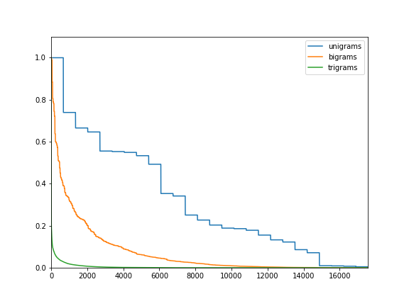 Unigrams have the advantage of being easy to calculate. But when we come to transposition ciphers (where the message is encrypted by changing the order of the letters), the unigram counts will stay the same. For these ciphers, 2-, 3-, 4-, or higher n-grams are useful. The disadvantage of longer n-grams is that the rarer n-grams occur very much less frequently (see figure to the right, showing relative frequency of unigrams, bigrams, and trigrams for English; click the image for a larger version). This means you may not see many (or any!) of each n-gram in your training set, meaning that things can go wrong when you're trying to break new messages.
But, if you can get away with it, larger n-grams are generally better for breaking ciphers.
Implementing n-grams
How do you find n-grams? With a little bit of string slicing:
def ngrams(text, n):
    return [text[i:i+n] for i in range(len(text)-n+1)]
Frequency counts as vectors
The bag of letters model is just a list of counts of each letter in some text. An ordered list of numbers is the same as a one-dimensional array, or a vector. For the vectors we're interested in, they're vectors in a 26-dimensional space.
For example, the text hello there can be represented as the vector:
| A | B | C | D | E | F | G | H | I | J | K | L | M | N | O | P | Q | R | S | T | U | V | W | X | Y | Z |
|---|---|---|---|---|---|---|---|---|---|---|---|---|---|---|---|---|---|---|---|---|---|---|---|---|---|
| 3 | 2 | 2 | 1 | 1 | 1 |
(there are zeros in the blank spaces, which I've left out for clarity) and the text the cat sat on the mat can be represented as:
| A | B | C | D | E | F | G | H | I | J | K | L | M | N | O | P | Q | R | S | T | U | V | W | X | Y | Z |
|---|---|---|---|---|---|---|---|---|---|---|---|---|---|---|---|---|---|---|---|---|---|---|---|---|---|
| 3 | 1 | 2 | 2 | 1 | 1 | 1 | 1 | 5 |
Mathematicians know a lot about vectors, and aren't fazed by high-dimensional spaces. We shouldn't be either.
Vectors can be thought of as being points in a space. If we're trying to find the similarity between two vectors, we can think about that as finding the distance between those two points. Mathematicians have thought a lot about vectors and distances, so we can use some of their techniques here.
The first thing to consider is that different length texts will have different numbers of letters and therefore represent points that are different distances away from the origin. That means we need to scale these vectors so that all the vectors are the same length; this kind of scaling is called normalising.
Once we have all the vector the same length, we have to find the distance between two points: one that represents the text we're looking with, the other being a representation of typical English. The closer these points, the more like English is the text we're concerned with.
Mathematicians have many ways of finding these distances, and use the term norm to generalise the idea of distance. The norm of a vector \(\mathbf{x}\) is written \(|\mathbf{x}|\) or \( \lVert \mathbf{x}\rVert \).
 If we're taking a geometric view of vectors (which we could if we're thinking about texts in alphabets with two or three letters, corresponding to vectors in two or three dimensional space), an obvious way to find lengths and distances is with Pythagoras's theorem; this is also called the Euclidean norm.
\[ |\mathbf{x}| = \sqrt{x_a^2 + x_b^2 + x_c^2} \]
where \(x_a\) is the number of as, \(x_b\) is the number of bs, and \(x_c\) is the number of cs (see the figure to the right). If the alphabet has more letters, the formula remains the same, but just with more terms in the square root.
 Another way of finding the length of a vector is the Manhattan distance or taxicab distance, named because it's the distance travelled going from here to here if you took a taxi across the grid structure of Manhattan (see left).
\[ |\mathbf{x}| = x_a + x_b + x_c \]
But, you can rewrite that equation as
\[ |\mathbf{x}| = \sqrt[1]{x_a^1 + x_b^1 + x_c^1} \]
That suggests you could measure distance with another variation:
\[ |\mathbf{x}| = \sqrt[3]{x_a^3 + x_b^3 + x_c^3} \]
and so on. And indeed you can. These collectively are known as the \( L_p \) norms, where p is the power used. The Euclidean norm is the \( L_2 \) norm; the Manhattan distance is the \( L_1 \) norm.
As the power p increases, the largest component of x gets to be more and more significant to the final norm value. Eventually, that gives us the \( L_\infty \) norm of
\[ L_\infty \thinspace \mathbf{x} = \max_i x_i \]
The \( L_0 \) just counts how many dimensions are non-zero. It's also called the Hamming distance and is generally only interesting with binary-valued dimensions, when it's a count of how many bits are different.
Implementing norms
Now we understand norms, how do we get Python to implement them?
First of all, we want to use the same basic function to do the two related jobs:
- find the "length" of a vector, which we can use to scale it to the correct length
- find the distance between two vectors.
The core of all this is the \(L_p\) norm, which we'll implement as a Python function lp. If we pass it one vector, it finds the length of it. If we pass it two vectors, it will find the distance between them. If p is unspecified, we'll use a values of p=2.
def lp(v1, v2=None, p=2):
    """Find the L_p norm. If passed one vector, find the length of that vector.
    If passed two vectors, find the length of the difference between them.
    """
    if v2:
        vec = {k: abs(v1[k] - v2[k]) for k in (v1.keys() | v2.keys())}
    else:
        vec = v1
    return sum(v ** p for v in vec.values()) ** (1.0 / p)
Note that v1.keys() returns a Set-like thing, so we use the set union operator | to combine the keys from both vectors.
Once we have that, all the other specific norms become easy:
def l1(v1, v2=None):
    return lp(v1, v2, 1)

def l2(v1, v2=None):
    return lp(v1, v2, 2)

def l3(v1, v2=None):
    return lp(v1, v2, 3)

def linf(v1, v2=None):
    if v2:
        vec = {k: abs(v1[k] - v2[k]) for k in (v1.keys() | v2.keys())}
    else:
        vec = v1
    return max(v for v in vec.values())
Scaling a vector needs to know which norm is being used, then just divides each component of the vector by that length.
def scale(frequencies, norm=l2):
    length = norm(frequencies)
    return collections.defaultdict(int,
        {k: v / length for k, v in frequencies.items()})
Again, the dimension-specific scales are defined in terms of scale:
def l2_scale(f):
    return scale(f, l2)

def l1_scale(f):
    return scale(f, l1)
Finally, give an easier name for the \(L_1\) and \(L_2\) norms:
normalise = l1_scale
euclidean_distance = l2
euclidean_scale = l2_scale
Cosine distances
 The final way of finding the difference between two vectors doesn't depend on normalising their lengths. Instead, the cosine distance looks at the angle between two vectors. The cosine is used because it's easy to calculate from the components of the two vectors:
\[ \text{similarity} = \cos(\theta) = {\mathbf{x} \cdot \mathbf{y} \over |\mathbf{x}| |\mathbf{y}|} = \frac{ \sum\limits_{i=1}^{n}{x_i y_i} }{ \sqrt{\sum\limits_{i=1}^{n}{x_i^2}} \sqrt{\sum\limits_{i=1}^{n}{y_i^2}} } \]
This gives the similarity of the vectors: a larger value means the vectors are closer. A cosine distance is just 1 minus the cosine similarity.
Implementing cosine distance
The cosine similarity and distance come direct from the definition.
def cosine_similarity(frequencies1, frequencies2):
    """Finds the distances between two frequency
    profiles, expressed as dictionaries.
    """
    numerator = 0
    length1 = 0
    length2 = 0
    for k in frequencies1.keys():
        numerator += frequencies1[k] * frequencies2[k]
        length1 += frequencies1[k]**2
    for k in frequencies2:
        length2 += frequencies2[k]**2
    return numerator / (length1 ** 0.5 * length2 ** 0.5)
That's more than enough for now. In Part 2 of this post, I'll look at how we can test which of these norms is the best when it comes to breaking ciphers.
Code
The code for this post is in either support.norms or support.language_models.
Acknowledgements
- The bigram and unigram counts files
count?.txt, came from Peter Norvig's page on letter count resources - Post cover photo from Tim Evans on Unsplash